Advent of Code 2023 - Day 23A Long Walk

| Problem statement | Source code | Tags: MazeGraph theoryBFS/DFSManual inspection

Part 1

The first realization is that most positions in the maze don't matter: since we can only visit each position once, if we are in a one-directional corridor, we have no choice but to go through it. So we can simplify the maze by collapsing these corridors into single edges. The only positions that matter are:

1. The start and end positions.
2. Positions with multiple enter/exit paths, which have wall neighbor number not equal to 2.
3. Slopes, because they can only be traversed in one direction, so from the other direction they are effectively walls.

This reminds of 2019 day 18, where we also simplified the maze by collapsing corridors.

Anyway, this is an entirely unremarkable (by the standards of day 23) algorithm. I first extract all such junction points (which just requires looking at the cell and its neighbors' values; no traversal required). Then I walk from each exit direction of each junction point until I hit another junction point (the path is unique along the way), and record the distance between them. This gives me a graph of junction points and their distances.

(By the way, there was a minor hiccup with producing these graphs: turned out that DiagrammeR doesn't work well with graphs containing name, so I have to delete the names before converting to DiagrammeR.)

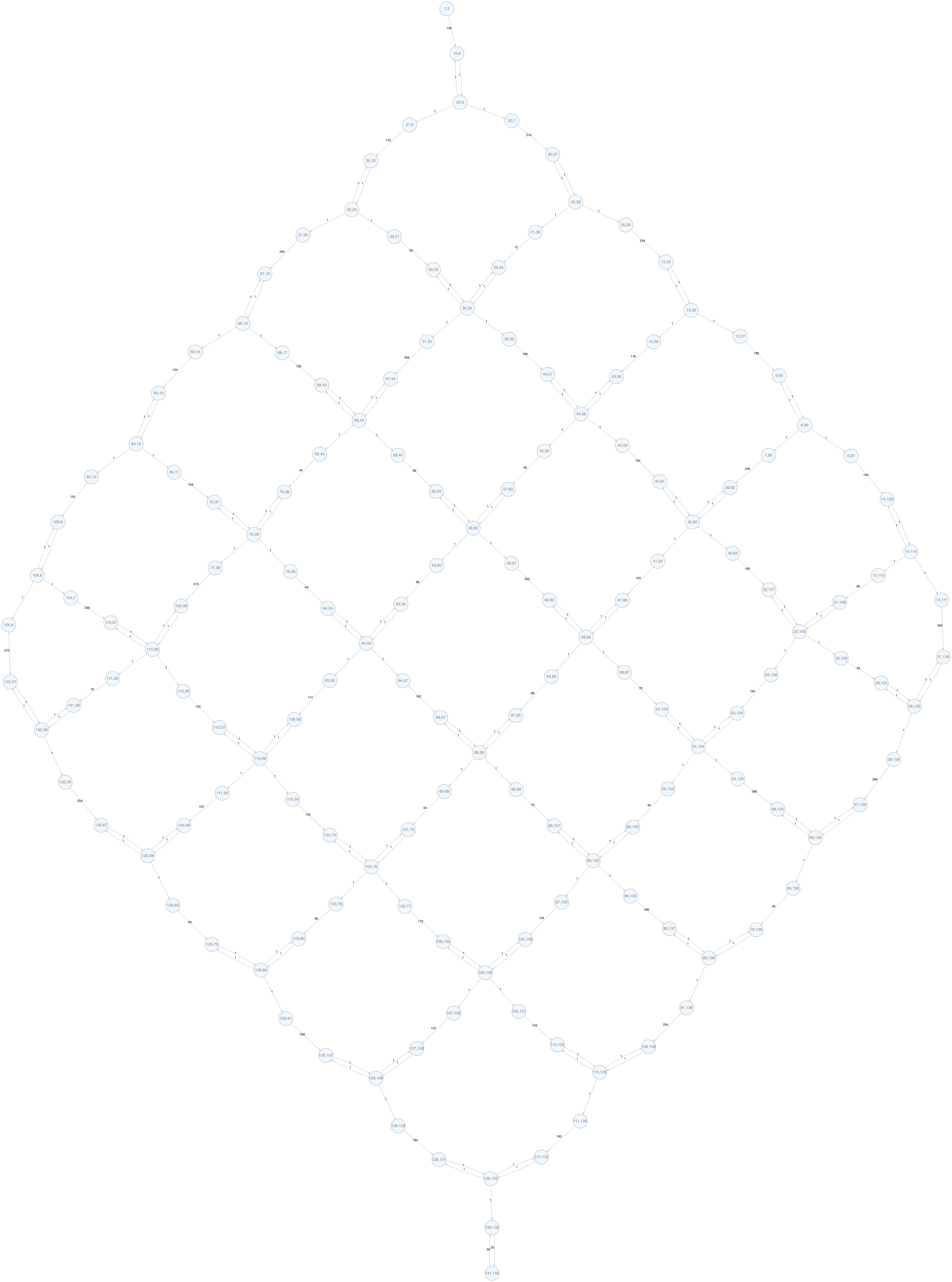
There's already something we can see from this graph, but it's still a bit too bloated. If we look at the path from one junction point to another, it looks like A -> B -> C <-> D. B is obviously useless because there's a single way to go from A to C; C is also useless because it can only be exited in one direction, so it must be entered from the other direction. So we can prune these nodes and get the following graph:

This is a grid graph where each edge points to the target node. (There are two triangles in the corners, but if you add an extra node in the middle of those edges, you get a regular grid graph.) Because it's a DAG, we can do a topological sort and then do a DFS (see longest path).

longest_path_dag <- function(graph, start_id, end_id) {
  topo <- igraph::topo_sort(graph, mode = "out")
  dist <- rep(-Inf, igraph::vcount(graph))
  dist[start_id] <- 0
  for (u in topo) {
    if (!is.finite(dist[u])) {
      next
    }
    out_edges <- igraph::incident(graph, igraph::V(graph)[u], mode = "out")
    if (length(out_edges) == 0) {
      next
    }
    targets <- igraph::ends(graph, out_edges, names = FALSE)[, 2]
    dist[targets] <-
      pmax(dist[targets], dist[u] + igraph::E(graph)[out_edges]$length)
  }

  dist[end_id]
}

Part 2

After removing the slopes, now all edges are bidirectional, so essentially the graph is the same but undirected:

However! Longest paths in undirected graphs are NP-hard, including in grid graphs. So a naïve DFS solution would be very slow. Let's start with the ill-performing version as a baseline. It enumerates every single path from the start to the end, of which there are 1,262,816, by adding one edge to the path at a time, and keeping track of the longest path length found so far. It uses a visited set to avoid cycles, which is reset when backtracking.

longest_path <- function(graph, start_id, end_id) {
  # Get adjacency list for DFS
  el <- igraph::as_edgelist(graph, names = FALSE)
  e_len <- igraph::edge_attr(graph, "length")
  n <- igraph::vcount(graph)

  neighbors <- vector("list", n)
  edge_lens <- vector("list", n)
  for (i in seq_len(n)) {
    neighbors[[i]] <- integer(0)
    edge_lens[[i]] <- numeric(0)
  }

  for (k in seq_len(m)) {
    u <- el[k, 1]
    v <- el[k, 2]
    w <- e_len[k]
    neighbors[[u]] <- c(neighbors[[u]], v)
    edge_lens[[u]] <- c(edge_lens[[u]], w)
    neighbors[[v]] <- c(neighbors[[v]], u)
    edge_lens[[v]] <- c(edge_lens[[v]], w)
  }

  visited <- rep(FALSE, n)
  visited[start_id] <- TRUE
  st <- stack()
  st$push(list(vertex = start_id, neighbor = 1, len = 0))
  max_len <- 0
  while (st$size() > 0) {
    fr <- st$pop()
    u <- fr$vertex
    i <- fr$neighbor

    # Done with this vertex, backtrack
    if (i > length(neighbors[[u]])) {
      if (u != start_id) {
        visited[u] <- FALSE
      }
      next
    }

    st$push(list(vertex = u, neighbor = i + 1, len = fr$len))
    v <- neighbors[[u]][i]
    if (visited[v]) {
      next
    }

    new_len <- fr$len + edge_lens[[u]][i]
    if (v == end_id) {
      max_len <- max(max_len, new_len)
      next
    }
    visited[v] <- TRUE
    st$push(list(vertex = v, neighbor = 1, len = new_len))
  }

  max_len
}

The above function ran in 3 minutes. I understand that R itself is slow and the above is not optimized, but any language-level optimizations won't help much.

Let's think about how we can prune branches. Although the number of paths from one corner to the other is few (1 million, as aforementioned), a lot of the times the algorithm made a decision that traps it in a dead end, but it doesn't know that until it has exhausted all paths within that dead end. So one optimization is to check if a vertex is a dead end before going into it. However, if we do a BFS for every branch, this just blows up the time by another factor of 36, and it's not immediately clear how deeply we can prune the search space. Instead, I implemented a heuristic: if we are at the edge of the grid, we can only go towards the end and never away from it, because otherwise we trap ourselves:

This also includes another case, which is if we are at the vertex right outside the end ("138,132" in the diagram), we have to go into the end, because if we leave it, we won't be able to come back again.

An edge node can be detected by counting its number of neighbors. I start from the end node, and trace the edge nodes back to the start node. Then in the DFS, if we are at an edge node, we don't consider the neighbor that is farther from the end node.

longest_path <- function(graph, start_id, end_id) {
  # ...
  # Precompute the distance from each edge node to the end node
  edge_node_dist_to_end <- rep(Inf, n)
  visited <- rep(FALSE, n)
  q <- queue()
  q$push(end_id)
  edge_node_dist_to_end[end_id] <- 0
  visited[end_id] <- TRUE
  while (q$size() > 0) {
    u <- q$pop()
    for (i in seq_along(neighbors[[u]])) {
      v <- neighbors[[u]][i]
      if (length(neighbors[[v]]) == 4 || visited[v]) {
        # Not an edge node
        next
      }
      visited[v] <- TRUE
      edge_node_dist_to_end[v] <- edge_node_dist_to_end[u] + 1
      q$push(v)
    }
  }
  # ...
  while (st$size() > 0) {
    # ...
    if (visited[v]) {
      next
    }
    # We are traveling away from the end, which would trap ourselves
    if (
      is.finite(edge_node_dist_to_end[v]) &&
        is.finite(edge_node_dist_to_end[u]) &&
        edge_node_dist_to_end[v] >= edge_node_dist_to_end[u]
    ) {
      next
    }

    # ...
  }

  max_len
}

This reduced the runtime to 40s, a 4.5x improvement. It's still not great though; for one thing, it can't detect dead ends that are not on the edge:

There's a second optimization, which is an upper-bound heuristic (similar to 2022 day 19). Since each node can contribute at most 1 in-edge and 1 out-edge to the path, the maximum remaining path length from $u$ to $e$ is given by

Where $\text{best1}[v]$ is the length of the longest edge from $u$, and $\text{best2}[v]$ is the length of the two longest edges from $v$. The extra factor of 1/2 is because we have double-counted each edge, once for each of its endpoints. If $\mathit{curBest} - \mathit{curLen}$ is larger than this upper bound, then we can never beat the current best, so we can prune this branch. This is paired with another trick: sort the neighbors by descending edge length, so that we are more likely to find a good path early on.

for (k in order(e_len, decreasing = TRUE)) {
  u <- el[k, 1]
  v <- el[k, 2]
  w <- e_len[k]
  neighbors[[u]] <- c(neighbors[[u]], v)
  edge_lens[[u]] <- c(edge_lens[[u]], w)
  neighbors[[v]] <- c(neighbors[[v]], u)
  edge_lens[[v]] <- c(edge_lens[[v]], w)
}

# ...

best1 <- rep(-Inf, n)
best2 <- rep(-Inf, n)
for (u in seq_len(n)) {
  best1[u] <- edge_lens[[u]][1]
  best2[u] <- if (length(edge_lens[[u]]) > 1) sum(edge_lens[[u]][1:2]) else 0
}

# ...
while (st$size() > 0) {
  # ...
  remaining_upper_bound <- best1[v] +
    best1[end_id] +
    sum(best2[!visited & seq_along(best2) != v & seq_along(best2) != end_id])
  if (new_len + remaining_upper_bound <= max_len) {
    next
  }
  visited[v] <- TRUE
  st$push(list(vertex = v, neighbor = 1, len = new_len))
}

How many paths did this prune? From 1,262,816 to 40,806, a 97% reduction! It reduces the runtime to 3s, another 13x improvement.

There's another optimization I could consider, which is memoization of the longest path from the start node to each node with a given visited set; then, if I encounter the same node and visited set again but with a shorter path (for example, because I already tried A,B,C,D and now trying A,C,B,D), I can immediately prune. However, because again, R is extremely bad with hash tables, I really didn't bother.